Graphs as a mathematical concept
Graphs are defined as a pair \(G = (V, E)\) were \(V\) is a set of vertices, and \(E\) is an unordered collection of pairs of vertices, called edges, for example: \(G = (\{a, b, c\}, [(a,b), (b,c), (c,a)])\)
Directed and undirected graphs
-
In undirected graphs, the edge pair indicates that both vertices are connected to each other
-
In directed graphs, the edge pair indicates that the first vertex is connected to the second, but not vice versa
| Term | Description |
|---|---|
| Adjacent Vertices | Vertices with an edge between them |
| Edges incident on a vertex | Edges which both connect to the same vertex |
| End vertices/endpoints | The two vertices in the pair that an edge connects to |
| Degree of a vertex | The number of edges that connect to a pair |
| Parallel edges | Two edges both connecting the same nodes (This is the reason why edges are an unordered collection, not a set) |
| Self-loop | An edge whose vertices are both the same |
| Path | A sequence of alternating vertices and edges, starting and ending in a vertex |
| Simple paths | Paths containing no repeating vertices (hence are acyclic) |
| Cycle | A path starting and ending at the same vertex |
| Acyclic | A graph containing no cycles |
| Simple cycle | A path where the only repeated vertex is the starting/ending one |
| Length (of a path of cycle) | The number of edges in the path/cycle |
| Tree | A connected acyclic graph |
| Weight | A weight is a numerical value attached to each edge. In weighted graphs relationships between vertices have a magnitude. |
| Dense | A dense graph is one where the number of edges is close to the maximal number of edges. |
| Sparse | A sparse graph is one with only a few edges. |
Graph properties
Property 1. The sum of the degrees of the vertices in an undirected graph is an even number.
Proof. Handshaking Theorem. Every edge must connect two vertices, so sum of degrees is twice the number of edges, which must be even.
Property 2. An undirected graph with no self loops nor parallel edges, with number of edges \(m\) and number of vertices \(n\) fulfils the property \(m \leq \frac{n \cdot (n-1)}{2}\)
Proof. The first vertex can connect to \(n-1\) vertices (all vertices bar itself), then the second can connect to \(n-2\) (all the vertices bar itself and the first vertex, which it is already connected to), and so on, giving the sum \(1+2+...+n\) , which is known to be \(\frac{n \cdot (n-1)}{2}\)
Fully connected graphs fulfil the property \(m = \frac{n \cdot (n-1)}{2}\)
Graphs as an ADT
Graphs are a “collection of vertex and edge objects”
They have a large number of fundamental operations, to the extent it is unnecessary to enumerate them here, but they are essentially just accessor, mutator, and count methods on the vertices and edges
Concrete Implementations
Edge List Structure
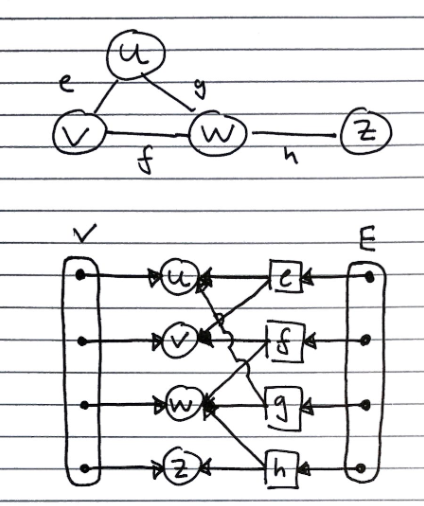
Consists of
- A list of vertices – contains references to vertex objects
- A list of edges – contains references to edge objects
- Vertex Object
- Contains the element that it stores
- Also has a reference to its position in the vertex list.
- Edge Object
- Contains the element it stores
- Reference to origin vertex
- Reference to destination vertex
- Reference to position in edge list
Advantage of Reference to Position. Allows faster removal of vertices from the vertex list because vertex objects already have a reference to their position.
Limitations. As you can see, the vertex objects has no information about the incident edges. Therefore, if we wanted to remove a vertex object, call it w, from the list we will have to scan the entire edge list to check which edges point to w.
Adjacency list
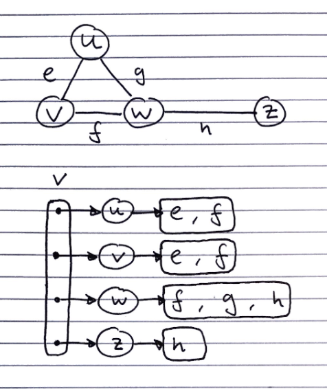
Consists of
- 1 list containing all of the vertices. Each of which have a pointer to a list edge objects of incident edges.
Adjacency matrix
This is an extension of the edge list structure – we extend/add-on to the vertex object.
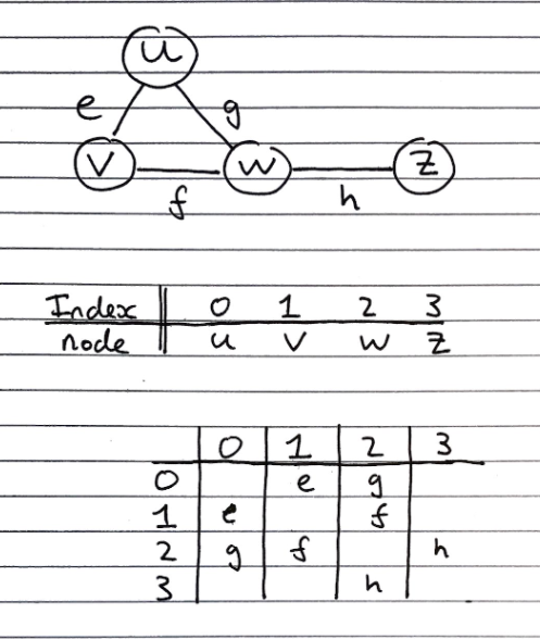
Consists of
- Extended/augmented Vertex Object
- Integer key (index) associated with each vertex. A graph with \(n\) vertices then their keys go from 0 to \((n-1)\).
- Adjacency Matrix – 2D Array
- Square matrix, with each dimension being the number of vertices \(n\)
- Let \(C_{ij}\) represent a particular cell in the matrix. \(C_{ij}\) either has a reference to an edge object for adjacent vertices or null for non-adjacent vertices.
- If a reference to an edge object, \(k\), is stored at cell \(C_{ij}\) it means that \(k\) is an edge from the vertex with index \(i\) to the vertex with index \(j\).
- If our graph is undirected then the matrix will be symmetrical across the main diagonal, meaning \(C_{ij} = C_{ji}\) (as shown in the diagram above).
Advantage of 2D Adjacency Array. We are able to lookup edges between vertices in \(O(1)\) time.
Limitations.
- Not easy to change the size of the array
- Space Complexity is \(O(n^2)\) and in many practical applications the graphs we are considering do not have many edges, so using an adjacency matrix might not be so space efficient.
Performance
Given a graph with n vertices and m edges (no parallel edges and no self-loops).
| Edge List | Adjacency List | Adjacency Matrix | |
|---|---|---|---|
| Space | O(n+m) | O(n+m) | O(n2) ❌ |
incidentEdges(v) |
O(m) | O(deg(v)) ⭐ | O(n) |
areAdjacent(v,w) |
O(m) | O(min(deg(v), deg(w))) | O(1) ⭐ |
insertVertex(o) |
O(1) | O(1) | O(n2) ❌ |
insertEdge(v,w,o) |
O(1) | O(1) | O(1) |
removeVertex(v) |
O(m) | O(deg(v)) ⭐ | O(n2) |
removeEdge(e) |
O(1) | O(1) | O(1) |
Space complexity (choosing between an adjacency matrix and an adjacency list)
We can determine more specific space complexities for both graph structures based on the type of graph we are using:
| Type of graph | Adjacency matrix | Adjacency list |
|---|---|---|
| General case | \(O(n^2)\) | \(O(n+m)\) ⭐ |
| Sparse | Inefficient use of \(O(n^2)\) space ❌ | Few edges to search through list for ⭐ |
| Dense | Efficient use of \(O(n^2)\) space ⭐ | Many edges to search through list for ❌ |
| Complete directed, with self-loops | \(O(n^2)\) ⭐ | \(O(n^2)\), and inefficient lookup ❌ |
Subgraphs
A subgraph of the graph \(G\) fulfils the two properties:
Its vertices are a subset of the vertices of \(G\)
Its edges are a subset of the edges of \(G\)
A spanning subgraph contains all of the vertices in \(G\). This then gives rise to spanning trees, which are spanning subgraphs which are connected and acyclic.
- A spanning tree is not unique unless the graph is a tree.
Depth-first search
Depth-first search is a general technique for traverse graphs. It takes \(O(n + m)\) time to search a graph of \(n\) vertices and \(m\) edges.
Informally, it can be described as always proceeding to its first adjacency, then backtracking when it reaches a vertex with no adjacencies which it has not explored already
Algorithm DFS(G,v):
    Input: A graph G and a vertex v of G
    Output: Labelling of edges of G in the connected component of v as discovery edges and back edges
        setLabel(v, "visited")
        for all e in G.incidentEdges(v)
            if getLabel(e) = "unexplored"
                // Get vertex w, that's opposite vertex v across edge e
                w <- opposite(v,e)
                if getLabel(w) = "unexplored"
                    setLabel(e, "discovery")
                    DFS(G,w) // Recursive call to DFS on this "unexplored" vertex w
                else
                    setLabel(e, "back")
It has the following properties
- It visits all vertices and edges in any connected component of a graph
- The discovery edges form a spanning tree of any graph it traverses
- The depth-first search tree of a fully connected graph is a straight line of nodes
Uses Cases
It can be used for path-finding by performing the traversal until the target node is found, then backtracking along the discovery edges to find the reverse of the path.
- This is done by altering the DFS algorithm to push visited vertices and discovery edges as the algorithm goes through them.
- Once the target vertex is found, we return the path as the contents of the stack
It can be used to identify cycles, as if it ever finds an adjacency to a vertex which it has already explored, (a back edge), the graph must contain a cycle.
- A stack is again used for the same purpose.
- When a back edge is encountered between a node v and another node w, the cycle is returned as the portion of the stack from the top to until node v.is
Breadth-first search
Breadth-first search is a technique to traverse graphs. It takes \(O(n + m)\) time to search a graph of \(n\) vertices and \(m\) edges.
Informally, it can be described as exploring every one of its adjacencies, then proceeding to the first adjacency, then backtracking when it reaches a vertex with no adjacencies which it has not explored already
Algorithm BFS(G)
    Input: graph G
    Output: Labelling of edges and partition of the vertices of G
    for all u in G.vertices()
        setLabel(u, "unexplored")
    for all e in G.edges()
        setLabel(e, "unexplored")
    for all v in G.vertices()
        if getLabel(v) == "unexplored"
            BFS(G,v)

Algorithm BGS(G,s)
    L0 <- new empty sequence
    L0.addLast(s)
    setLabel(s, "visited")
    while !L0.isEmpty()
        Lnext <- new empty sequence
        for all v in L0.elements()
            for all e in G.incidentEdges(v)
                if getLabel(e) = "unexplored"
                    w <- opposite(v,e)
                    if getLabel(w) = "unexplored"
                        setLabel(e, "discovery")
                        setLabel(w, "visited")
                        Lnext.addLast(w)
                    else
                        setLabel(e, "cross")
        L0 <- Lnext // Set L0 to Lnext so while loop won't stop
It has the following properties
- It visits all vertices and edges in \(G_s\), the connected component of a graph \(s\)
- The discovery edges form a spanning tree of any graph it traverses
- The path between any two vertices in the spanning tree of discovery edges it creates is the shortest path between them in the graph
- The bread-first search tree of a fully connected graph is like a star with the centre node being the starting node, and all other nodes being rays, with the only vertices being from the starting node to all other nodes
It can be used for path-finding by performing the traversal until the target node is found, then backtracking along the discovery edges to find the reverse of the path.
It can be used to identify cycles, as if it ever finds an adjacency to a vertex which it has already explored, (a back edge), the graph must contain a cycle.
Applications
We can specialise the BFS algorithm to solve the following problems in \(O(n+m)\) time.
- Compute the connected components of G
- Compute a spanning forest of G
- Find a simple cycle in G, or report that G is a forest
- Given two vertices of G, find a path in G between them with the minimum number of edges, or report that no such path exists.
DFS and BFS visualization
The site linked here traces the steps of DFS either or BFS, and one can specify whether each node is connected, as well as whether the graphs are directed or undirected