Rational Agents

Rational Agents

In a rational agent a goal can be specified by some performance metric.

A rational agent will choose the the actions that maximizes the expected value.

Inputs to an agent

• Abilities A set of actions that the agent can perform
• Goal What is the agent trying to achieve
• Prior Knowledge What sis the agent kno when it came into being
• History
• • Stimuli: The current environment
• • Past experiences

Agent System

An agent systems is an agent in an environment

receives **stimuli** and caries out **actions**

Dimensions of an Agent

An agent can be defined in many ways or dimensions that specifies its complexity and structure.

Modularity

How is the agent structured

• Flat Agent has one level.
• Modules Agent has many interlinking modules.
• Hierarchy Agent has a hierarchy(recursive) of modules.

Planning horizon

How far ahead is the agent expected to plan

• Static World does not change.
• Finite Stages The agent plans a finite number of steps.
• Indefinite The agent plans a finite but unknown number of steps.
• Infinite The agent plans continuously.

Representation

How is the environment represented

• Explicit states A state is one of the ways the world can be.
• Features or Propositions States can be described using features.
• Individuals and relations Feature of relationships between sets of individuals.

  Computational limits

  How is the agent limited by computation

• Perfect rationality The agent can determine the best course of action.

• Bounded rationality The agent must make a good decision with computation and memory limitations.

Learning from experience

does the agent learn form experience

• Knowledge is given at creation.
• Knowledge is learnt from past experiences.

Sensing uncertainty

How well does the agent know its environment

• Fully observable The agent knows its entire environment.
• Partially observable There is a limited number of states, the observation is nto true to reality.

Effect uncertainty

Cant the result of an effect be known

• Deterministic The resulting state can be known form the previous state and action.
• Stochastic There us uncertainty about the environment after the action.

Preference

What is the agents desire

• Achievement goal The agent must reach a goal which could be the result of a complex formulae.
• Complex preferences The agent has a range of complex preferences that interact with one another.
• • Ordinal Only the order of the preferences matters.
• • Cardinal The value of the preferences matters.

Number of Agents

• Single Agent All other agents are part of the environment.
• Multiple Agent Agents will reason about the actions of other.agents

Interaction

How does the agent interact with the environment

• Reason offline reason before taking action.
• Reason online reason while taking action.

Representation

To compute a problem the problem must be in a computable representation before an output can be provided

Requirements

An representation should be

• Rich enough to express the knowledge needed
• As close to the problem as possible
• Amenable to efficient computation
• Able to be acquired

Solution

Quality of a solution

• Optimal Solution The best solution possible
• Satisfactory solution A solution that is good enough
• Approximate solution A solution that is close to an optimal solution
• Probable solution A solution that is likely to be correct

Decisions and Outcomes

Good decisions can have bad outcomes and Bad decisions can have good outcomes

Information can lead to better decisions.

Computation time can provide a better solution.

An Any time algorithm an produce a solution at any time but given more computation time the solution gets better

A worse solution now maybe be better than an optimal solution later.

Physical symbol Hypothesis

A symbol is a physical pattern that can be represented.

A symbol-system has the means to manipulate symbols.

hypothesis a Physical symbol system has the means for general intelligent action

Knowledge and symbol levels

• Knowledge level : Agent’s knowledge, beliefs and goals.
• Symbol level Describes what reasoning agent does. This is what the agent uses to implement the knowledge level

Abstraction

• Low level Easier for machines to understand
• High level Easier for humans to understand

Reasoning and acting

• Design time reasoning and computation Reasoning done by designer to design the agent.
• Offline computation Done by agent before it has to act
• Online computation Done by agent “on the go”

  Knowledge base and observations

• Knowledge base Compiled background knowledge and data
• Observations Information obtained online
• Both used to make decisions

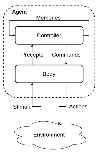
Agent Architectures

Agent architectures

Body

The agent interacts with the environment through the body

The body:

• Perceives stimuli form the environment and creates precepts for the controller
• Receives commands form the controller and generates actions on the environment
• In some cases may have actions that are not controlled

Controller

The controller is the brains of the agent and generates commands based on current and previous precepts. Controllers have a limited memory and computational resources

Agent logic

Traces

• Percept Trace A sequence of all percepts, past present and future.
• Command Trace A sequence of all commands, past present and future.
• Agent History A sequence of past and present commands and precepts at to time \(t\).
• transduction A function from percept traces to command traces.
• History Percepts to time \(t\) (including time \(t\)) + Commands to time \(t\) = History at \(t\)
• Causal transduction History at time \(t\) -> Command at \(t\)
• Controller An implementation of a causal transduction.

Belief Status

An agent has limited memory

It must decide what subset of its history to remember

This is the agents memory

At every step the controller needs to decide

1. What to do
2. What to remember

A belief status should approximate the environment

Single level hierarchy

In a single level hierarchy the agent has one body and a single controller.

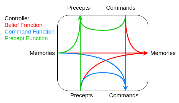
functions

• Belief state function controls the next belief state / memories.
• Command state function decides on the commands the controller should produce.

Advantages

Simpler and can be easier to program

Disadvantages

All problems are processes together, e.g collision detection and long term planning

This can slow down the goals that need a quick response time

Multi level hierarchy

Made from a body and many layers of controllers.

Each controller acts as a virtual body to the controller above. It receives precepts and commands from the controller below it and sends selected precepts and commands to the controller above.

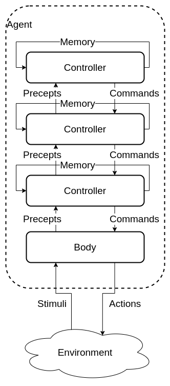
functions

• Belief state function controls the next belief state / memories.
• Command state function decides on the commands the controller should produce.
• Precept function decides what commands to send to the higher controller

Agent Types

Ideal Mapping

In principle an agent can be though of as an mapping from the set of precepts to the set of commands. There is a theoretical Ideal mapping where the ideal action is taken at each step. The simple approach would be a lookup table:

• Table too large
• Time to build

The goal of an agent is to approximate this ideal mapping

Simple Reflex agents

Simple agents based on a series of if -> else statements

Can achieve fairly complex behavior.

Can be run quickly

Reflex agent with State

similar to the simple Reflex Agents but retains knowledge

Needs an internal state

Can keep track of a changing world

Goal based agents

Keeps track of what is trying to be achieved

More flexible than a reflex agent

Utility based agents

Uses a Utility function to judge the state of the world

Allows for a choice of which goals to achieve and can select the one with the highest utility.

If goal outcomes are uncertain a probability formula can be used.

Learning Agent

Adds in several components

• critic Using a performance standard informs the learning agent how well it is doing.
• performance element responsible for acting based on the improvements from the learning agent.
• learning element responsible for making improvements with knowledge of the agents success.
• problem generator responsible for suggesting actions for new experiences to attempt to prevent being stuck at a local maximum

Takes information about hove the performance agent is doing and attempts to optimise the agent to improve performance. Learning provides the agent with autonomy.

Problem Formulation

Problem formulation

Given a specification of a solution, not an algorithm to follow

Agent has a a starting state and wants to get to the goal state

Many problems can ba abstracted into the problem of finding a path in a directed graph.

Problem solving steps

• Goal Formulation Identify a desirable solution
• Problem formulation - identify the problem
• Search find the sequence of actions
• Execution Perform the actions

types of Environment

• Deterministic, Fully observable
  • The agent knows everything about the current state
  • The agent knows what state the environment will be in after any action
• Deterministic, Partially observable
  • The agent has limited access to the current state
  • The agent can determine a set of states from a given action
  • Instead of actions on a single state the agent must manipulate sets fo states
• Stochastic, partially Observable
  • The agent has limited access to state
  • The agent does not know the effect of any action
  • Must use sensors to determine an effect
  • Search and executions are interwoven
• Unknown state space
  • Knowledge is learned
  • (not a priority in the module)

State Space Problem

• Has a set of states \(S\)
• Start states A Subset of states where the agent can start
• action function Given a state and an action returns the new state
• goal states A subset of states that the agent targets
• A criterion that specifies the quality fo a solution

Abstraction

The real world is complex and so abstraction is uses

Abstract states are a subset of real states

Abstract operations are a combination of real actions

Abstract Solution A set of paths between states that are applicable to the real world

State space graph

A state space problem can be represented using a stat space graph

A state space graph consists of a set \(S\) of \(N\) nodes and a set of orders pairs \(A\) representing arcs or edges

if \(<S_i,S_j> \in S\) then \(S_i\) is a neighbor to \(S_j\)

A path is a sequence of nodes \(<n_1,n_2,n_3....n_i>\) such that \(<n_{i-1},n_i> \in S\)

Given a set of start and and nodes a solution is a path from a start node to an end node.

To solve these problems the ability to navigate a tree or graph is very useful.

Uninformed Search

Getting from a to b on a simple directed graph with no prior knowledge

following an informed search through a graph can simulate th exploration fo the state space

Tree Search

Algorithm

The exploration of an uninformed tree search tends follows the following algorithm.

node <- Root or starting node
goal <- a target goal
frontier <- some data store


frontier.add(node)
while (items in frontier){
    current= frontier.RemoveTop()
    if (current==goal){
        return current
    }
    for (neighbor of current){
        frontier.push(neighbor)
    }
}
return none <- no solutions found

• node An element in a graph, continuing a parent and actions needed to reach its children
• frontier the nodes currently explored the type of data structure depends on the algorithm

Graph Search

With tree search state space with loops give rises to repeated states that cause inefficiencies.

Graph search is a practical way of exploring a state space that can account to such repetitions.

Rather than holding nodes in the frontier a graph search instead holds the path of nodes needed to reach the current point in the frontier.

node <- Root or starting node
goal <- a target goal
frontier <- some data store


frontier.add([node])
while (items in frontier){
    current= frontier.RemoveTop()
    if (current[last]==goal){
        return current
    }
    for (neighbor of current[last]){
        current.add(neighbor)
        frontier.push(current)
    }
}
return none <- no solutions found

Analysis

An algorithm can be judged by different metrics

• Completeness can the solution be found
• optimality does the solution find the solution with the least cost
• Complexity
  • Judged by several factors
    • b Maximum branch factor
    • d Depth of least cost
    • m maximum depth can be infinite
  • time complexity how does the time taken scale
  • space complexity how many nodes in memory

Breath first

A queue is used for the frontier data store

Prioritizes expanding horizontally over expanding vertically

Complexity

• completeness will always find a solution if b is finite

• time \(1 + b + b^2 +b^3 +...+ b^d = O(b^d)\)

• space \(1 + b + b^2 +b^3 +...+ b^d = O(b^d)\)

• Optimal Yes if cost is a function of depth, not optimal in general

Space complexity is the biggest issue with this type of search

Depth first

A stack is used for the frontier data store Prioritizes expanding vertically over expanding horizontally

Complexity

• completeness Fails with infinite depth or loops
  • can be modified to avoid loops
• time \(1 + b + b^2 +b^3 +...+ b^d = O(b^d)\)

• space \(1 + b + b^2 +b^3 +...+ b^d = O(bm)\)

• Optimal No

Not optimal but cuts down on space complexity a lot

Lowest Cost First

A priority queue is used for the frontier data store where the key is the cost of the path.

The cost of a path is the current is the sum of the cost of each of it’s arcs.

The path of least cost is chosen first from the frontier to expand.

When arc costs are equal simply produces a breath first search.

Comparison

|Strategy|Frontier Selection|Complete|Halts| Space | |-|-|-|-|-| |Breadth-first| First node added| Yes | No | Exp| | Depth-first | Last node added | No | No | Linear| | Lowest cost first| minimal cost | Yes | No | Exp|

• complete- Guaranteed to fins a solution if one exists.
• Halts - on a finite graph (maybe with cycles).
• Space as a function of the length of the current path.

Informed Search

Using information about the goal to inform our path choice.

Heuristic

Extra information used to guide the path is called a heuristic

The heuristic \(h(n)\) is th estimated minimum cost to get form a node to the goal node

Calculating \(h(n)\) needs to be done efficiently

A \(h(n)\) function is an underestimate if there is no path from the node \(n\) to the goal with cost strictly less than \(h(n)\)

A heuristic is admissible if it is both:

• A non-negative function
• An underestimate of the actual cost

Best First Search

We can use the heuristic to determine the order fo the stack representing the frontier.

Select the path that is closest to the goal node, according to the heuristic function.

Greedy best-first search selects a path on the frontier with the lowest heuristic value.

A priority queue is used as the frontier.

This algorithm can get stuck in loops.

Complexity

Space: \(b^n\) where b is the branching factor and n is the path length

Time: \(b^n\)

Not guaranteed to find a solution

It does nto always find te shortest path

A* Search

A* search uses a combination os path cost and heuristic value to guess the length of a path too the goal if a particular node is chosen.

[f(p) = {cost}(p) + h(p)]

The frontier is a priority queue sorted by the \(f(p)\) function

The node on the frontier with the lowest estimated cost from the start to the goal via such node is chosen.

A* search is admissable if:

• The branching factor is finite
• Arc costs are bounded above Zero
• the function \(h(n)\) is non-negative and is an underestimate fo the shortest path of n to the goal node

Proof

It can be shown that the A* algorithm is admissable.

Let \(P\) be a path selected from the frontier to the goal node.

Suppose path \(P'\) is on the frontier, because \(P\) was selected before \(P'\) and \(h(p) =0\) \(cost(P) \leq cost(P') + h(P')\)

Because h is an underestimate \(cost(P') + h(P') \leq cost(P'')\) For any path \(P''\) that extends \(P'\) So \(cost(P) \leq cost(P'')\) for any path \(P''\) to a goal

Solution

Theorem: A* will always find a solution if there is one

The frontier always contains the initial part of a path to a goal

As A* runs the costs of the paths keeps increasing and will eventually exceed any finite number.

Admissability does nto guarantee that every node selected from the frontier is on an optimal path but that the first solution found wil be optimal even with graphs with cycles.

Heuristics

The performance of the A* algorithm depends on the performance of the heuristic, given a path \(P\) and a heuristic function \(h\) and \(c\) is the cost of the optimal solution the heuristic can fall into 3 categories.

\(cost(p) + h(p) \lt c\)(1) \(cost(p) + h(p) = c\)(2) \(cost(p) + h(p) \gt c\)(3)

A* expands all paths in the set \(\{cost(p) + h(p) \lt c\}\)

A* expands some paths in the set \(\{cost(p) + h(p) = c\}\)

Increasing the heuristic while keeping it admissable reduces the size of the sets.

Complexity

time: exponential in relative error of \(h*\) Length of solution

space: Exponential keeps all nodes in memory

Comparison

|Strategy|Frontier Selection|Complete|Halts| Space | |-|-|-|-|-| |Breadth-first| First node added| Yes | No | Exp| | Depth-first | Last node added | No | No | Linear| | Heuristic-depth-first | local min \(h(p)\)| No | No | Linear| | Best-first | Global min \(h(p)\)| No | No | Linear| | Lowest cost first| minimal cost | Yes | No | Exp| | A*| minimal \(f(p)\) | Yes | No | Exp|

• complete- Guaranteed to fins a solution if one exists.
• Halts - on a finite graph (maybe with cycles).
• Space as a function of the length of the current path.

Search Optimizations

Cycle Checking

The search encounters a node on a path that it has already encountered (the path traversed a cycle)

Solution

Prune the path as it is not an optimal path so does not need to be explored

Implementation

Keeping the nodes in the path in a hash table allows for checking in constant \(O(1)\) time.

Multiple Path Pruning

Two paths may meet at the same note, one taking a longer path anther a shorter one.

Solutions

• If the expanding path is shorter it can be pruned
• Otherwise if the expanding path \(<s,..n>_1\) is shorter than the current path \(<s,..n,..m>_2\) for subpath \(<s,..n>_2\) then
  • Employ a strategy to prevent this from happening
  • Remove all paths from the frontier that include subpath \(<s,..n>_2\)
  • Change the initial segment of the paths on the frontier to use the shorter path. All paths containing \(<s,..n>_2\) has the subpath replaced with \(<s,..n>_1\)

Implementation

Maintain a set of explored set (closed list) of nodes.

Initially the closed list is empty

When a path is selected if the endpoint in the closed list then a conflict has emerged otherwise add the endpoint to the closed list.

Implementation with A*

Suppose path \(p'\) to \(n'\) was selected but there is a lower cost path to \(n'\) Suppose this is via point \(p\) on the frontier.

let path \(p\) end at node \(n\)

by A* \(p'\) was selected before \(p\) i.e \(f(p')<f(p)\)

[cost(p’) + h(p’) \leq cost(p)+h(p)]

The path of \(n'\) via \(p\) is lower cost than via \(p'\)

[cost(p)+ cost(n,n’) \lt cost(p’)]

[cost(n,n’) \lt cost(p’)- cost(p) \leq h(p) -h(p’) = h(n)-h(n’)]

we can ensure that this does not occur if

[\vert h(n) - h(n’) \vert \leq cost(n,n’)]

The heuristic is a monotone restriction

Monotone Restriction

A heuristic function satisfies the monotone restriction if \(\vert h(m) - h(n) \vert \leq cost(m,n)\) for every arc \(<m,n>\)

If h satisfies the monotone function is is consistent meaning \(h(m) \lt cost(m,n) + h(n)\)

A* with a consistent heuristic and multiple path pruning always finds the shortest path to a goal

Direction of a Search

A search can be thought of as symmetric

Shortest path from start to end

equals

Shortest path from end to start

Forward branching factor number of arcs that are leaving ths node

Backwards branching factor number of arcs that are entering ths node

Search complexity is b^n so use forward is forward branching factor \(\lt\) backwards branching factor.

However when a graph is dynamically constructed the backwards graph may not be available.

Bi-directional Search

Search backwards from the goal and the start simultaneously

This can be effective since \(2b^{k/2} \lt b^k\)

Implementation can vary however one strategy is to do a breath first stack to generate a rangd of targets then to do anther strategy like depth first to find the most optimal strategy.

Island Driven Search

This process expands on the idea of multiple hops to many hops between islands.

Find a set of m islands between the start and end.

There are m smaller problems \(mb^k/m \lt b^k\)

There are issues to overcome:

• Identifying island can be difficult
• Hard to guarantee optimality

Dynamic Programming

For statically stored graphs, build a table of dist(n) the actual distance form node n to a gaol

This can be build backwards from the goal:

This can be used locally to determine what to do

There are two main problems

• It requires enough space
• The dist function needs to be recomputed for each goal

Bounded Depth-first search

A bounded depth first search takes a bound (cost or depth) and does nto exceed paths that exceed the bound

• Explores part of the search graph
• Uses space linear in the depth of the Search

Iterative-deepening search

• start with a bound b=0
• Do a bounded depth-first search with bound b
• If a solution is found return that solution
• Otherwise, increment b and repeat

Finds the same first solution as breadth first search.

As is based on depth first uses linear space.

Iterative deepening has an overhead of \((\frac{b}{b-1}) *\) cost of expanding nodes at depth \(k\).

When \(b=2\) there is an overhead factor of \(2\) when \(b=3\) there is an overhead of \(1.5\) as b gets higher, the overhead factor reduces.

Depth-first Branch-and-Bound

Combines depth-first search with heuristic information and finds the optimal solution.

Most useful when there are multiple solutions and we want an optimal one.

Uses the space of depth-first search.

let bound be the lowest-cost path found to a goal.

If the search encounters a path p where \(cost(p)+h(p) \geq bound\) the path can be pruned.

If a non - pruned path to the goal is found then bound can be set to \(cost(p)\) and p is set to the best solution.

Initializing Bound

• Bound can be initialized to \(\infty\)
• Bound can be set to an estimate of the optimal path cost
• After depth-first search terminates either
  • A solution was found
  • No solution was found and no path was pruned
  • No solution was found and a Path was pruned

Can be combined with iterative deepening to increase the bound until either a solution is found or to show there is no solution

Heuristics

The choice of a heuristic to choose can have a large impact in the efficiency and running time of the search.

Characterizing Heuristics

Def: If an A* tree-search expands N nodes and solution depth is d, then the effective branching factor b*, is the branching factor a uniform tree of depth d would have to contain N nodes.

[N = 1 + b* + (b)^2 + .. + (b)^d]

It is desirable to obtain a branching factor as close to one as possible, a smaller branching factor allows a larger problem to be solved.

We can estimate b* experimentally and it is usually consistent when performed over multiple runs.

If the branching factor of one heuristic is smaller then it should be used.

More specifically if

[h_1(n) \geq h_2(n) \forall n]

then \(h_1\) dominates \(h_2\)

A* expands all nodes with \(f(n) <f*\) where \(f*\) is the cost of the optimal path. All nodes with \(h(n)\lt f*=g(n)\) expanded

An admissable heuristic with higher values is better.

The computation for the heuristic should be taken into account as well.

Deriving heuristics

Relaxed problems

Admissible heuristics can be derived from a relaxed problem.

A relaxed problem is obtained by reducing the restrictions on operations.

e.g

• Get from the start node to the end node by traversing the graph
• Get from the start node to the end node

If there are several heuristics and none dominate then the maximum heuristic from the set may be chosen for any given value of \(n\), more formally:

[h(n) = max(h_1(n) , h_2(n) …)]

Pattern Databases

Store exact solution costs for each possible sub problem instance.

Heuristic \(h_{DB}\) = cost of solution ot corresponding subproblem.

Construct database by searching backwards from goal.

Other approaches

• Statistical approaches
  • Gather probable heuristics from training problems
  • e.g if \(95%\) of all cases \(cost(n,goal)\) is 20 then \(n(n)=20\)
  • Not admissable but still likely to expand less
• Select Features of a state to contribute to the heuristic
  • e.g For Chess number/ type of pieces left
  • Can use learning to determine weighting